Model fitting

Fitting procedure

SourceXtractor++ can fit models to the images of detected objects. The fit is performed by minimizing the loss function

(3)\[\lambda(\boldsymbol{q}) = \sum_i \left(g\left(\frac{p_i - \tilde{m}_i(\boldsymbol{q})}{\sigma_i}\right)\right)^2 + \sum_j \left(\frac{f_j(\boldsymbol{q}) - \mu_j}{s_j}\right)^2\]

with respect to components of the model parameter vector \(\boldsymbol{q}\). \(\boldsymbol{q}\) comprises parameters describing the shape of the model and the model central coordinates \(\boldsymbol{x}\).

Modified least squares

The first term in (3) is a modified weighted sum of squares that aims at minimizing the residuals of the fit. \(p_i\), \(\tilde{m}_i(\boldsymbol{q})\) and \(\sigma_i\) are respectively the pixel value above the background, the value of the resampled model, and the pixel value uncertainty at image pixel \(i\). \(g(u)\) is a derivable monotonous function that reduces the influence of large deviations from the model, such as the contamination by neighbors (Fig. 3):

(4)\[g(u) = u_0\,\mathrm{arsinh}\,\frac{u}{u_0}.\]

\(u_0\) sets the level below which \(g(u)\approx u\). In practice, choosing \(u_0 = \kappa \sigma_i\) with \(\kappa = 10\) makes the first term in (3) behave like a traditional weighted sum of squares for residuals close to the noise level.

Caution

The cost function in (3) is optimized for noise distributions with a Gaussian core and makes model-fitting in SourceXtractor++ appropriate only for image noise with a pdf symmetrical around the mean.

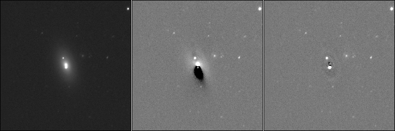
Fig. 3 Effect of the modified least squares loss function on fitting a model to a galaxy with a bright neighbor. Left: the original image; Middle: residuals of the model fitting with a regular least squares (\(\kappa = +\infty\)); Right: modified least squares with \(\kappa = 10\).

The vector \(\tilde{\boldsymbol{m}}(\boldsymbol{q})\) is obtained by convolving the high resolution model \(\boldsymbol{m}(\boldsymbol{q})\) with the local PSF model \(\boldsymbol{\phi}\) and applying a resampling operator \(\mathbf{R}(\boldsymbol{x})\) to generate the final model raster at position \(\boldsymbol{x}\) at the nominal image resolution:

(5)\[\tilde{\boldsymbol{m}}(\boldsymbol{q}) = \mathbf{R}(\boldsymbol{x}) (\boldsymbol{m}(\boldsymbol{q})*\boldsymbol{\phi}).\]

\(\mathbf{R}(\boldsymbol{x})\) depends on the pixel coordinates \(\boldsymbol{x}\) of the model centroid:

(6)\[\mathbf{R}_{ij}(\boldsymbol{x}) = h\left(\boldsymbol{x}_j - \eta.(\boldsymbol{x}_i - \boldsymbol{x})\right),\]

where \(h\) is a 2-dimensional interpolant (interpolating function), \(\boldsymbol{x}_i\) is the coordinate vector of image pixel \(i\), \(\boldsymbol{x}_j\) the coordinate vector of model sample \(j\), and \(\eta\) is the image-to-model sampling step ratio (sampling factor) which is by default defined by the PSF model sampling. We adopt a Lánczos-4 function [11] as interpolant.

Configuring model-fitting

The model-fitting process can be precisely defined and tuned in the measurement configuration Python script.

Model parameters

In SourceXtractor++, any of the model parameters \(q_j\) may be a constant parameter, a free parameter, or a dependent parameter.

Constant parameters

In the model fitting configuration, constant parameters are declared using the ConstantParameter() construct:

size = ConstantParameter(42)

One can also use a lambda expression based on actual measurements for the current object:

size = ConstantParameter(lambda o: 2 * o.get_radius())

Free parameters

Free parameters are adjusted by minimizing \(\lambda(\boldsymbol{q})\) in (3). They are declared using the FreeParameter() construct. The free parameter initial value follows the same rules as the constant parameter value: it may be defined as a simple number supplied by the user, e.g.:

size = FreeParameter(42, range)

or as a lambda expression, such as:

size = FreeParameter(lambda o: 2.5 * o.get_radius(), range)

Many model parameters are valid only over a restricted domain. Fluxes, for instance, cannot be negative. The purpose of the range argument is to define the boundaries of the domain. In SourceXtractor++, this domain restriction is achieved through a change of variables, applied individually to every model parameter:

(7)\[q_j = f_j(q^\mathsf{(min)}_j, q^\mathsf{(max)}_j, Q_j).\]

The “model” variable \(q_j\) is bounded by the lower limit \(q^\mathsf{(min)}_j\) and the upper limit \(q^\mathsf{(max)}_j\) by construction. The “engine” variable \(Q_j\) can take any value, and is actually the parameter that is being adjusted in the fit, although it does not have any physical meaning.

Parameter range

The Range() construct is used to set \(q^\mathsf{(min)}_j\), \(q^\mathsf{(max)}_j\), and \(f_j()\):

range = Range((-1,1), RangeType.LINEAR)

The first argument is a tuple of 2 numbers specifying the lower and upper limits of the range. The range type defines \(f_j()\). Currently supported range types are linear (RangeType.LINEAR) and exponential (RangeType.EXPONENTIAL). Linear ranges are appropriate for parameters such as positions or shape indices. Exponential ranges are better suited to strictly positive parameters with a large dynamic range, such as fluxes and aspect ratios:

range = Range((0.01,100), RangeType.EXPONENTIAL)

The relation between model and engine parameters is plotted Fig. 4 for both examples. Table 1 details the formula applied for currently supported range types.

Fig. 4 Engine vs model parameters. Left: example of a linear range (x position parameter in the range \(]-1, 1[\)). Right: example of an exponential range (aspect ratio parameter in the range \(]0.01,100[\)). Note the logarithmic scale of the abcissa in the second example.

Table 1 Types of changes of variables applied to model parameters

Type	Model \(\stackrel{f^{-1}}{\to}\) Engine	Engine \(\stackrel{f}{\to}\) Model	Examples
Unbounded (linear)	\(Q_j = q_j\)	\(q_j = Q_j\)	Position angles
RangeType.LINEAR	\(Q_j = \ln \frac{q_j - q^\mathsf{(min)}_j}{q^\mathsf{(max)}_j - q_j}\)	\(q_j = \frac{q^\mathsf{(max)}_j - q^\mathsf{(min)}_j}{1 + \exp -Q_j} + q^\mathsf{(min)}_j\)	positions Sersic index
RangeType.EXPONENTIAL	\(Q_j = \ln \frac{\ln q_j - \ln q^\mathsf{(min)}_j}{\ln q^\mathsf{(max)}_j - \ln q_j}\)	\(q_j = q^\mathsf{(min)}_j \frac{\ln q^\mathsf{(max)}_j - \ln q^\mathsf{(min)}_j}{1 + \exp -Q_j}\)	fluxes aspect ratios

In practice, we find this approach to ease convergence and to be much more reliable than a box constrained algorithm [12].

Predefined free parameters

SourceXtractor++ comes with two pre-defined free parameters for easily initializing positions (get_pos_parameters()) and fluxes (get_flux_parameter()):

def get_pos_parameters():
  return (
      FreeParameter(lambda o: o.get_centroid_x(), Range(lambda v,o: (v-o.get_radius(), v+o.get_radius()), RangeType.LINEAR)),
      FreeParameter(lambda o: o.get_centroid_y(), Range(lambda v,o: (v-o.get_radius(), v+o.get_radius()), RangeType.LINEAR))
  )

def get_flux_parameter(type=FluxParameterType.ISO, scale=1):
  func_map = {
      FluxParameterType.ISO : 'get_iso_flux'
  }
  return FreeParameter(lambda o: getattr(o, func_map[type])() * scale, Range(lambda v,o: (v * 1E-3, v * 1E3), RangeType.EXPONENTIAL))

Note the use of lambda functions in the first argument to Range().

Dependent parameters

It is often useful to define dependencies between parameters. Dependent parameters are declared using the DependentParameter() construct. For instance, one may wish to adjust the sizes of two components of a model in parallel:

size1 = FreeParameter(lambda o: 2 * o.get_radius(), Range((0.01, 100.0), RangeType.EXPONENTIAL))
size2 = DependentParameter(lambda s: 1.2 * s, size1)

Parameter dependencies are useful for computing new output columns from fitted parameters:

MAG_ZEROPOINT = 33.568
mag = DependentParameter(lambda f: -2.5 * np.log10(f) + MAG_ZEROPOINT, flux)

Parameter dependencies may also be used to apply changes of variables for setting complex priors, as we shall see in the next section.

Models

The full models \(\boldsymbol{m}(\boldsymbol{q})\) are defined as a sum of one or several 2D functions. These model components are added using the add_model() function. For instance, for adding a point source model component one may insert

add_model(group, PointSourceModel(x, y, flux))

Composite models (e.g., a galaxy bulge plus a disk component) may be generated by inserting multiple add_model() with the same measurement group. Model components need not be coaxial.

SourceXtractor++ currently supports the following models.

Constant: ConstantModel

This is the simplest model, which applies a constant offset to the image:

(8)\[\boldsymbol{m}_{\tt Constant} = m_0\]

Point source: PointSourceModel

The point source model is appropriate for representing unresolved sources such as stars. It is a scaled delta function, and as such depends only on a coordinate vector \(\boldsymbol{r} = (x, y)\) and a flux \(m_0\).

(9)\[\boldsymbol{m}_{\tt POINTSOURCE}(\boldsymbol{r}) = m_0 \delta(\boldsymbol{r})\]

Sérsic: SersicModel

The Sérsic model has an elliptical shape with aspect ratio \(\rho\) and position angle \(\theta\), and a Sérsic profile [13] with effective radius \(R_e\) and Sérsic index \(n\):

(10)\[m_{\tt Sersic}(r) = m_0 \exp \left(- b(n)\,\left({R\over R_e}\right)^{1/n}\right),\]

where \(b(n)\) is the solution to

(11)\[2 \gamma[2\,n,b(n)] = \Gamma(2\,n)\]

An accurate approximation for the solution to \(b(n)\) in (11) is [14]:

\[b(n) = 2\,n - {1\over3} + {4\over 405\,n} + {46\over 25515\,n^2} + {131\over 1148175\,n^3}\]

Exponential: ExponentialModel

The exponential model is a Sérsic model with fixed \(n=1\). It is generally appropriate for describing galaxy disks.

de Vaucouleurs: DeVaucouleursModel

The de Vaucouleurs model is a Sérsic model with fixed \(n=4\). It can be a good fit to elliptical galaxies and galaxy bulges.

Regularization

Although minimizing the (modified) weighted sum of least squares gives a solution that fits best the data, it does not necessarily correspond to the most probable solution given what we know about celestial objects. The discrepancy is particularly significant in very faint (SNR \(\le 20\)) and barely resolved galaxies. For instance, there is a tendency to overestimate the elongation of such galaxies, known as the “noise bias” in the weak-lensing community [15, 16, 17, 18]. The second term in (3) implements a simple Tikhonov regularization scheme to mitigate this issue. This penalty term acts as a Gaussian prior on the selected (free or dependent) parameters.

Priors are inserted using the add_prior() function. For instance, one can put a Gaussian prior on the flux, centered on the initial isophotal guess from the detection image, with a 10% standard deviation:

flux = get_flux_parameter()
add_prior(flux, lambda o: o.get_iso_flux(), lambda o: 0.1 * o.get_iso_flux())

Non-Gaussian priors

Sometimes a Gaussian prior is unsuited to some parameters (e.g., to disfavor excessively low or high values, but not both). In that case a change of variable must be applied. This is easily accomplished using a dependent parameter. For example, to penalize Sérsic index values \(n\) above \(n_0\), one can apply the change of variable:

(12)\[N = e^{n - n_0},\]

which can be implemented as (assuming \(n_0=4\) and a Gaussian prior on \(N\) centered on 0 with unit standard deviation):

n = Freeparameter(2.0, Range((0.3, 8.0), RangeType.LINEAR))
n0 = 4
nc = DependentParameter(lambda nt: np.exp(nt - n0), n)
add_prior(nc, 0.0, 1.0)

Fig. 5 shows the resulting prior on \(n\) , and its regularizing effect on the solution.

Fig. 5 Effect of a non-Gaussian prior generated through a change of variable (see text). Left: Effective prior on the Sérsic index. Right: Distribution of Sérsic indices obtained for Sérsic fits on noisy data before (blue) and after (green) applying the prior.

Caution

Although any function valid over the parameter range could in principle be used for the change of variable, only functions producing concave priors are likely to play nice with the current minimization algorithm and lead to consistent results.

Combinations of parameters

Priors are also useful for penalizing some values taken by specific combinations of parameters. For example, the following code applied to images taken in the \(g\) and \(r\) bands sets a Gaussian prior on the color index \(g - r\) of the detected point sources (centered on \(g - r = 0.5\), with standard deviation 0.3):

...
MAG_ZEROPOINT = 32.19
flux_g = get_flux_parameter()
flux_r = get_flux_parameter()
mag_g = DependentParameter(lambda f: -2.5 * np.log10(f) + MAG_ZEROPOINT, flux_g)
mag_r = DependentParameter(lambda f: -2.5 * np.log10(f) + MAG_ZEROPOINT, flux_r)
col = DependentParameter(lambda g,r: g - r, mag_g, mag_r)
add_prior(col, 0.5, 0.3)

group_g = mesgroup['g']
group_r = mesgroup['r']
add_model(group_g, PointSourceModel(x, y, flux_g))
add_model(group_r, PointSourceModel(x, y, flux_r))
add_output_column('mag_g', mag_g)
add_output_column('mag_r', mag_r)
...

Fig. 6 shows the impact of the prior on the color-magnitude diagram.

Fig. 6 Effect of a Gaussian prior (centered on 0.5 mag with standard deviation 0.3 mag) on \(g - r\) source color measurements.

Minimization

Minimization of the loss function \(\lambda(\boldsymbol{q})\) is carried out using the Levenberg-Marquardt algorithm. Two Levenberg-Marquardt engines are supported in the current version of SourceXtractor++: the LevMar library [19], and the GSL implementation. LevMar approximates the Jacobian matrix of the model from finite differences using Broyden’s [20] rank one updates, which results in less evaluations of the model and \(\approx\) 30% faster processing. The default engine is levmar, but can be switched to gsl if preferred using the set_engine() function, e.g.:

set_engine('gsl')

The fit is done inside a disk which diameter is scaled to include the isophotal footprint of the object, plus the FWHM of the PSF, plus a 20 % margin.

\(1\,\sigma\) uncertainty estimates are provided for most measurement parameters; they are obtained from the full covariance matrix of the fit, which is itself computed by inverting the approximate Hessian matrix of \(\lambda(\boldsymbol{q})\) at the solution.